Calculate Time In Minutes

LadyDi

Registered User.
Local time
Today, 13:56
Joined
Mar 29, 2007
Messages
894
I have a spreadsheet that lists service calls for one of our customers. That customer has several locations that my company services. My manager has asked me to set up a formula that will calculate the time in minutes between service calls for each location. My spreadsheet lists the location (a site number assigned to that location by my company), the date and time the call was completed (two separate columns), and the date and time the call was initiated (again, two separate columns). I need to look down this list find the locations that match and calculate the times between calls.

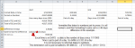
Here is an example of my spreadsheet:

Location -- Contact Date -- Contact Time -- Complete Date --Complete Time
1 ---------- 2/12/13 -------- 8:00 AM ------- 2/12/13 -------- 8:30 AM
2 ---------- 2/12/13 -------- 12:00 PM ------ 2/13/13 -------- 8:00 AM
1 ---------- 2/13/13 -------- 5:00 PM ------- 2/13/13 -------- 5:15 AM
2 ---------- 2/14/13 -------- 8:00 AM ------- 2/14/13 -------- 8:30 AM

I need to add a column that will show 1950 minutes for Location 1 and 1440 minutes for Location 2 (the minutes between the complete time of the first call to contact time of the second call). The locations will not be listed together. The calls go in consecutive order for the customer. Any assistance you can provide would be greatly appreciated.
 
assuming your start time is in a2 and your end time is in b2
=((B2-A2)*24)*60

...i think
 
Last edited:
Will that take into consideration if the calls are several days apart?
 
yes... it should

i think it is important that the start/end time cells are formatted

here are two examples i played with to check.
mm/dd/yyyy hh:mm:ss

stat time--------------end time------------length in mins
2/14/13 1:00 AM ------2/14/2013 1:30 -----30
2/14/13 1:00 PM ------2/15/13 2:00 PM ----1500
 
ahh i see youre date and time are in two separate columns.....

let me see about that


i think i got it!!


Complete date is E15
complete time is F15
Contact Date is b15
contact time is c15

=(((E15+F15)-(B15+C15))*24)*60

let me know if that doesnt work
 
Last edited:
Assuming your data is in columns A:E, then in F2 try:

=(LOOKUP(2,1/($A$2:$A$25=A2),$B$2:$B$25+$C$2:$C$25)-INDEX($D$2:$D$25+$E$2:$E$25,MATCH(A2,$A$2:$A$25,0)))*1440

adjust the ranges to cover your whole database (don't use too many more rows than necessary), then copy down.
 
Just add the (Date + time) - (Date1 + Time1) * 24 * 60 for minutes.

Attached and example.
You see, a Date is nothing more than the number of days since 1/1/1900 (different for Mac Excel). So, in the attached example I have a date and a time. The Time is nothing more than a fraction of the date.
How you choose to format it is for humans, but Excel sees it the same.

You can see that I copied the date and formatted it to a number on the example. The same for the time. So 8:00 AM = 0.333 days.

It is not necessary to reformat your date and times.
Simply add the Date Plus the Time - the other Date plus the Time
In the cell that displays the difference, simply change the format to HH:MM:SS
Oh, you wanted minutes - just format it in minutes.

In my example, the number was close to 2 1/2 days (i.e. 2.56181 days)
now take that number and use =B16*24*60 (24 hours * 60 minutes in an hour) - That would be the total number of minutes.
 

Attachments

  • Date format example.png
    Date format example.png
    31 KB · Views: 199
This is formula (=(LOOKUP(2,1/($N:$N=N2),$Z:$Z+$AA:$AA)-INDEX($AB:$AB+$AC:$AC,MATCH(N2,$N:$N,0) ))*1440) is really close. The only problem is that it calculates the number of minutes between the first and the last call, and there could be several calls in the middle that are not calculated. For Example, here is an example for one location -

01/11/13 8:31 PM 01/11/13 9:45 PM
01/12/13 9:05 AM 01/12/13 10:29 AM
01/13/13 4:41 PM 01/13/13 5:42 PM
01/16/13 3:29 PM 01/16/13 5:30 PM
01/20/13 11:39 AM 01/20/13 3:30 PM
01/22/13 8:45 AM 01/22/13 10:18 AM
01/24/13 8:32 AM 01/24/13 12:20 PM
01/28/13 7:38 PM 01/28/13 8:48 PM
01/29/13 7:43 AM 01/29/13 10:07 AM
02/04/13 11:05 AM 02/04/13 4:17 PM
02/07/13 3:00 PM 02/07/13 4:15 PM

I need to know the minutes between each consecutive call. If there is not a call after it, then there should not be any minutes showing. In other words, the last call should be blank in the new column. The first row of this table should show 680 minutes, the second row should show something like 1810 minutes, and the last row should be blank.

I tried using this formula ((Date + time) - (Date1 + Time1) * 24 * 60 ), but am having a problem with it because I need it to look down the list and find the next call for the same location - not just the next call.
 
How about?

=IFERROR((INDEX($B3:$B$25+$C3:$C$25,MATCH($A2,$A3:$A$25,0))-($D2+$E2))*1440,"")
 
This is great. I just have one problem. For some reason, it is not showing a blank when my site number changes. Instead, it shows a huge negative number (i.e. -39259). Do you know why that would be, and how I can correct it? Thank you so much for your help. I really appreciate it.
 
I am not seeing that issue. Can you illustrate?
 
I found a solution to this problem. By just adding an additional IF statement, I got it to skip the first call for each site.

=IF(N2=N3,IFERROR((INDEX($Z3:$Z$1000+$AA3:$AA$1000,MATCH($N3,$N3:$N$1000,0))-($AB2+$AC2))*1440,""), "")

Thank you so much for all of your help.
 

Users who are viewing this thread

Back
Top Bottom