Interactive chart data in Excel 365

[kilroyscarnival]

Recently we upgraded to Office 365 and I'm slowly exploring what's new in it. (Excited about the XLOOKUP and FILTER options!)

I've been tasked with creating some dynamic (interactive) charts with bulk amounts of Excel data (upwards of 1,000, perhaps sometimes 10,000 rows, and multiple columns. Ideally, the chart could be updated on the fly to a particular row range, and columns could be selected/deselected with checkboxes.

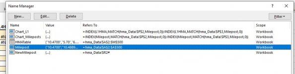
I started by turning my data into a table and creating named ranges out of the columns. From watching a few tutorials, I was able to get an INDEX:INDEX formula to give me the rows selected in two dropdown cells created by data validation on column A. I then created a named range using the Index(Match):Index(Match) formulas. But for whatever reason, when I go to paste or choose my named range into the horizontal axis field, it gives me a formula error.

Off I go searching for another solution. A different YouTuber used the spilled array itself as the named range; if my Index:Index formula was in $R$2, my spill array is $R$2#. I create that as a named range and the chart isn't taking that either. I tried it with and without the sheet name. (My working copy has the chart off to the right on the same page, but because this will be charting a lot of data, ultimately I will move the chart to its own sheet with a small dashboard.)

I have a feeling I'm missing something pretty basic, the equivalent of someone walking over and wordlessly taking the lens cap off my camera.

Attaching a zipped one-sheet workbook, on which I removed the named columns I had, just so the attempts at creating dynamic named ranges will be more easy to see. I also took a screenshot of my Name Manager display with the formulas. Somehow I feel maybe it was a mistake creating a table in the first place and I should have used plain data and plain cell references.

Thanks for any advice.

Ann

 

[Isaac]

Thanks for posting that about XLOOKUP. Where I am, many users are on 365 but some still on 2010. Still, that's a golden nugget I learned for soon-future use.

Question, have you fully explored the option of Pivot Charts? I mean, talk about dynamically adjusting a chart....they're pretty good for that.
And of course you can then use VBA, if desired, to manipulate them. That seems like the easiest way to me to get to a fairly interactive result. Haven't looked at your file yet.

 

[kilroyscarnival]

If only a pivot chart would meet this need. The data represents actual surface measurement of pavement thickness on a road, so they want the line chart to parallel the irregularities to indicate places where stress and wear are occurring, and be able to hone in on ranges (thus the dropdowns to specific mileposts, or in future, stationing (x##+00 labels). So in that case, summarizing the data wouldn't really do the trick.

As for XLOOKUP, it looks really easy, especially when your lookup and dependent columns might not be left-to-right oriented. Of course, Leila Gharani on YouTube makes a lot of things look easy. Most of the tutorials out there are still on older versions of Excel.

 

[Isaac]

If only a pivot chart would meet this need. The data represents actual surface measurement of pavement thickness on a road, so they want the line chart to parallel the irregularities to indicate places where stress and wear are occurring, and be able to hone in on ranges (thus the dropdowns to specific mileposts, or in future, stationing (x##+00 labels). So in that case, summarizing the data wouldn't really do the trick.

I see...kind of. If I have some time later I will download your file and check it out - maybe things will become clearer to me then.

But for now, taking this literally:

Ideally, the chart could be updated on the fly to a particular row range, and columns could be selected/deselected with checkboxes

.... Couldn't you populate comboboxes (or better yet multi-select listboxes) with the user-facing options (like which rows or columns to include in chart), and then simply use a line or two of VBA to update the chart's Data Source?

    Dim rng As Range
    Set rng = Thisworkbook.worksheets("Sheet1").Range(something)
    Thisworkbook.worksheets("Sheet1").ChartObjects("Chart 1").Chart.SetSourceData Source:=rng

 

[Isaac]

On second thought, this might be even easier.
I just noticed that if you have a chart based on columns A to D, and then you simply Hide columns B and C, the chart immediately updates....restructuring the entire visual, the Line and the Axis....according to col A and D only.

Maybe a multi select listbox where you select or deselect the col's and row's to hide?

 

[kilroyscarnival]

Isaac, thanks for all your thoughts!

I finally figured out what I guess I was doing wrong. I made the named ranges again in the same workbook, but as I was making them I chose the scope as "worksheet" rather than "workbook". So, my named range for the dynamic L1, "_L1", was 'hma_Data'!$S$2# to include the spilled values. NOW the chart will accept that named range for a series values. I redid all the others plus the milepost column, and it works.

Alternatively, maybe I needed to type in "='Sheetname'!" before the named range (in my case 'hma_Data!') but for some reason I thought the named range was the named range and didn't need the qualifier, especially because in this beginning stage, it's the only worksheet in the workbook. Ultimately, there will be other sheets because there will be other arrays.

Anyway, I really appreciate your thinking this through with me and also the VBA suggestions. I'm one of those ol' Excel hacks who basically only learned enough code to get by editing my recorded macros, though I'm really making a concerted effort to learn to write from scratch. I'm just not there yet. Any suggestions as to a good guide (book, class, video series, etc.) to help me along? I tried LinkedIn Learning's intro to VBA last year but got bored with it.

Adding a copy of my sheet with the chart now hopefully updating with the dropdown data in P23 changing. It is for me at least.

I feel like celebrating! At least with coffee and a peanut granola bar. This is a breakthrough on the step I was hung up on for a while.

I will have to go back and try your suggestion of hiding data columns to see what happens.

I may get stuck again, as this is going to have a lot of moving parts to it. The raw data is very clunky and so my first step is to pull all the similar data (in the case of this one, the HMA values) off to a separate spreadsheet, and replace the blank cells with N/A so that they don't chart as zeros. I may have eight separate charts in the end.

Thanks again for your time and considerate suggestions.

Best,

Ann

 

[Isaac]

Great, I'm glad to hear you got it working!

Any suggestions as to a good guide (book, class, video series, etc.) to help me along? I tried LinkedIn Learning's intro to VBA last year but got bored with it

I just learned from having projects and specific use cases for it (no books or tutorials), and me personally I could never see using videos to learn to code, (I feel like technical design is all about terminology so my preference is written), so unfortunately can't help you there.
I can offer a few general thoughts, though. These are just my humble opinion. And sometimes, just my opinion. LOL.

1. Don't use Select, Selection, Active and Activate in vba code. Ever. That is junk code which will eventually fail and when it does it will be very confusing and hard to troubleshoot, because it can present itself in 1000 different ways that will make it very unlikely you will realize what is actually happening. Everything may be good in testing, because you are one single person using one single workbook and sitting there patiently for your code to finish, giving it the best possible environment to run. When some user who normally has 15 excel workbooks open at a time (as any good little corporate minion does!), suddenly your program will crash and burn. What you meant to mean "what is selected on Sheet1 because nobody is touching the screen", suddenly becomes what a user has selected on Sheet5, or even Workbook2, at which point you may get "subscript out of range" (no sheet in the book), or "application or object-defined error" (you used offset(-1,0) after they'd unexpectedly selected range A1), or "cannot name a sheet..." (you tried to name something Sheet2 in the "active workbook" which turned out to be something else they had open already had a Sheet2)....the list is infinite. You'll never be able to replicate the error on your end because the cause is using vague code that could mean different things in different scenarios. Instead, declare variables (like Range, Worksheet, and Workbook) and SET those appropriately (like A1, Sheet2, and ThisWorkbook), then your code will never fail like that.
2. Remember that very much of the code you see on sites like MrExcel.com and Ozgrid is junk code like #1. Don't be swayed. Do it right and you'll be much better off
3. Remember that the macro recorder produces junk code also like #1...Edit all of it to use the appropriate references.
4. Know that the macro recorder will often produce code that reflects the most modern implementation of something according to the version you are on--So try to catch those things and fix them, i.e., if you are on a modern v. of 365 and record macro while doing a Sort, it will utilize the Add2 method, which doesn't exist in Excel 2010.
5. A few ideas of commonly utilized things to practice: Learn how to declare and set Workbook variables (i.e., = ThisWorkbook, =Workbooks.Open, =Workbooks("name of open book.xlsx"). To set Range variables (i.e., =wsVariable.Range("A1"), = rngVariable.offset(0,3), = rngVariable.Resize). To set Worksheet variables (i.e., =wbVariable.Worksheets("name"), =wbVariable.worksheets(#), = wbVariable.worksheets(wbVariable.Worksheets.count) [last sheet], = wbVariable.Worksheets.add(after:=wbVariable.Worksheets(wbVariable.Worksheets.count))

Have fun!