My knowledge of VBA for formatting and colouring cells is pretty ok, but I am struggling with the logic flows/loops especially in this situation where I want to colour rows in groups based on what is exported from a query.
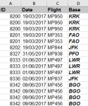
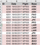
I have attached 2 images a before and after formatting which I would like to have applied.
The column which will drive the formatting is ID. This ID column will never export in a set pattern e.g odd, even, odd, even etc. As you can see from the images, there will be a varying number of rows which have the same ID. The total number of rows used by the export will also vary.
I have made it so my export groups together the IDs so at least that bit is sorted, but how would I go about coding it so that these rows are highlighted in an alternating but grouped pattern.
Thanks")
EDIT: From looking around on the internet, it seems as though the go to method is to use a helper column. I would rather not use this method as it seems inefficient and supposedly it is doable using conditional formatting + a named range. As my Excel data comes from an Access Query, the range comes in prenamed for me which is really useful. I have tried using the formula suggested in the last post found here https://stackoverflow.com/questions/4146822/excel-shading-entire-row-based-on-change-of-value, but can't seem to get it working. From what I understand all I need to do is to change CurrentRange with my named range (which is qry_reportPart_criteria) in the formula in the conditional formatting of =MOD(Fixed(SUMPRODUCT(1/COUNTIF(CurrentRange,CurrentRange))),2)=0
I have attached 2 images a before and after formatting which I would like to have applied.
The column which will drive the formatting is ID. This ID column will never export in a set pattern e.g odd, even, odd, even etc. As you can see from the images, there will be a varying number of rows which have the same ID. The total number of rows used by the export will also vary.
I have made it so my export groups together the IDs so at least that bit is sorted, but how would I go about coding it so that these rows are highlighted in an alternating but grouped pattern.
Thanks
EDIT: From looking around on the internet, it seems as though the go to method is to use a helper column. I would rather not use this method as it seems inefficient and supposedly it is doable using conditional formatting + a named range. As my Excel data comes from an Access Query, the range comes in prenamed for me which is really useful. I have tried using the formula suggested in the last post found here https://stackoverflow.com/questions/4146822/excel-shading-entire-row-based-on-change-of-value, but can't seem to get it working. From what I understand all I need to do is to change CurrentRange with my named range (which is qry_reportPart_criteria) in the formula in the conditional formatting of =MOD(Fixed(SUMPRODUCT(1/COUNTIF(CurrentRange,CurrentRange))),2)=0
Attachments
Last edited: