Copying colour in a formula

StephenSLR

Registered User.
Local time
Today, 14:47
Joined
Oct 25, 2005
Messages
48
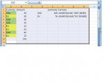
Is it possible to set a formula to copy a colour/format of a cell when it selects the values?

I have set up a sumif formula in a cell to select from a range of cells.

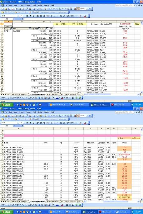
In the range I have coloured the cells containing the prices in USD of one company in Green and another company's prices in Euro in Yellow.

The sumif formula inputs the values rather well but not the formatting.

When I see the sumif summary I'd like a quick view of green vs. yellow

It is also an error check if I want to use USD values of Green company I can quickly spot a yellow cell meaning I have to change the exchange range.

s
 
I have to assume the rows contain the currency. Could you just use that?
I have attached an example? I'm probably way off with what you want, so could you supply an example of your own?
 

Attachments

  • sumif.jpg
    sumif.jpg
    32.1 KB · Views: 169
I'll try to explain, my spreadsheet is quite complicated.

In the top left corner of my sheet I'm using the formula

=SUMIF($H$124:$H$2180,H5,$Q$124:$Q$2180)

At the bottom of the sheet the H column has one set of data and the price is in the same row in the Q column.

I'm inputting values from 2 or 3 companies into the Q column and I'm colour coding the cells respectively.

When the results are calculated only the values appear in the top left part of my sheet. I'd like to see the formatting also appear so I can distinguish whose price it is.

Thanks for the help.

s
 
I may be way off track too, but have you considered using 'conditional formatting'? It can automatically set the colours for you based on the contents of other cells (such as the company).
 
An example of your spreadsheet would be useful, but I think I understand what you want and believe that it can only be achieved by code.

I assume that H5 contains criteria that is changed to get a sum in A1 from all values in Q124 etc where the value in H124 etc matches H5, and that the values in q col are colour coded and you want A1 to be that colour.

Use the worksheet change event.

Brian

Code:
Private Sub Worksheet_Change(ByVal Target As Range)

If Target.Address = "$H$5" Then

matchrow = Application.WorksheetFunction _
        .Match(Range("H5"), Worksheets("Sheet1").Range("H124:H2180"), 0)
With Worksheets("Sheet1")
     .Cells(matchrow + 123, 17).Copy    ' +123 to allow for starting row of array
     .Range("A1").PasteSpecial Paste:=xlPasteFormats
Application.CutCopyMode = False

End With

End If

End Sub
 
Last edited:
An example of your spreadsheet would be useful, but I think I understand what you want and believe that it can only be achieved by code.

excel.jpg


As you can see from the top image, column I has values taken from column Q in the bottom image. The values are transferred over but not the formatting.

I'm not sure how to use that code you pasted, if it can do what I want how do I put it into use?

Thanks for the help.

s
 
It was not what I expected, I'm not sure I understand, can you not attach your workbook as I have visual problems and cannot read the image clearly, plus it would help me try any code that I might develop.

Brian

Having squinted at this again are you sure that PaulJR's suggestion of conditional formatting isn't the answer.
 
Last edited:
can you not attach your workbook.

I've attached one page and edited it to keep the size small, the file is 12 Mb all up.

Don't refresh the pivot table as the pages it is linked to aren't included in the file.

Having squinted at this again are you sure that PaulJR's suggestion of conditional formatting isn't the answer

I'm not sure, conditional formatting from what I understand works if a value is below or above a certain number?

s
 

Attachments

I can't work out how you differentiate between the 2 companies in your spreadsheet - as you stated in your original email.

But I will confirm conditional formatting can set formatting based on words. Open the conditional formating box and change 'between' to 'formula' - then you can set the formatting based on characters or numbers that exist in another cell.

I'm not sure how this can help you though, as I can't see what you can filter on. I might be right in noticing a relationship between your colouring scheme and the schedule, although I'm not sure.
 
Last edited:
Like Paul i cannot see how you select the colour for your original list, it looks like hard work.

If it is just a case of knowing then I guess the only thing that you can do is run code from a command button on the spreadsheet or in the tool bar, in the code in the attached sheet the 3 named ranges are not dynamic and would need updating if data is added.
Note I added dat in H83 tohelp testing.

Also note that the error handling is basic it assumes all errors are a N/A return from the match.

Brian
 

Attachments

had a look at the attachment

could you not next to the price at the bottom have another column could be hidden for asthetics which had a symbol U or E signifying USD or Euro.

This column could be filled in using conditional formatting from the price column.

Then you could do a vertical lookup against the part number for the value of the cell. Have this in the cell next to the sum if.

Then use conditional formatting again to read this value but change the formatting of the cell to the right your sum if cell.

hope you understand.
 
I can't work out how you differentiate between the 2 companies in your spreadsheet.

I have coloured the prices of SPFA tan, e.g. (Q:137), the prices of Buhlmann have been coloured yellow e.g. (Q:158)

Let me explain.

When I receive a price list from SPFA I go to column H and match the prices to the pipe specs.

1 inch pipe of schedule 40 is in row 137

SPFA charge 7.23 per metre so I go to Q:137 and put in the price of 7.23 then I colour that cell tan.

The suppliers do not price every pipe and schedule.

Buhlmann have priced 6 inch pipe schedule 80 so I look for a match (or create one)

In this instance it is in row 158, I put in a formula to convert it into USD then colour that cell yellow.

It is a spreadsheet that was designed by my boss so I can't do a drastic reconstruction

The pivot tables select data from other pages, that I removed.

When you refresh the pivot tables the quantities within those tables change as well as the tables themselves, they compress or expand with new rows and values, however the values in column I remain static. Those values in column I will feed other values on another page to give total prices per tonne, etc.

I created the lower part of that page to make column I dynamic so it changes with the pivot table each time it is refreshed.

The formula in column I selects values from the Q column below. If you notice the value of I:5 = Q:137 but not the formatting. I would like the formula in column I to select the format as well as the value.

Then I can look beside the pivot table and see how many cells are yellow versus tan, then I will get a rough idea who has priced the most pipe for the job and it is preferable to get all the pipe from that supplier, at a glance if I see lots of yellow I will know the prices will be in EUR and the currency is a little more stable than the USD so it will not change by much in say a years time when the project kicks off.

I hope this is not too confusing.

s
 
I understand completely but I think dusty gave the answer. I would have another column alongside the price showing B or S as the supplier then instead of colouring per supplier enter B or S Conditional formatting can then do the colouring for both ranges.

I'm sure your Boss is not stupid and would allow such a simple and effective change.

Brian
 
I would like the formula in column I to select the format as well as the value.

I notice you have repeated this comment. We're not ignoring it, but I think you may have to dismiss it - I'm certain it's impossible to do in Excel.
 
I understand completely but I think dusty gave the answer. I would have another column alongside the price showing B or S as the supplier then instead of colouring per supplier enter B or S Conditional formatting can then do the colouring for both ranges.

Thanks, I think I understand.

In column R from row 111 downwards I'm putting an S or a B, etc. into the corresponding cell.

Then using conditional formatting in column J from row 4 down.
If the value = S colour cell tan, if the value = B colour cell yellow.

What formula is best to use in column J to match the value in column H from below and bring up the value (an S or B) from column R:111 downwards?

I tried the SUMIF formula that I used in column I but it only works if I use a numerical value for an S or B.

Thanks everyone for the help.

s
 
Formula for the conditional formatting is:

condition 1: =R111="S"
condition 2: =R111="B"

Put this formula in cell I4 first.

Then copy cell I4, and use paste special (select formats) to insert the conditional formatting from I5 to I83.

Does that help?
 
Yes Paul that will work there but for the top rows a far more complex Formula is required, also I notice that he has "est" in cell R152, to allow for that he would have to code =Left(R111,1)="B" .

I attach workbook with spreadsheet (2) showing conditions neededrows 152 and 64 allow for est to be included , if this is so then that has to be in all conditional formats, I use the Format painter (see help) to do this work.

Brian
 

Attachments

Sometimes one's mind gets stuck in a rut. Instead of Offset and Match I should have used Vlookup with range value of FALSE, after naming the necessary array.

=VLOOKUP(H4,condformatarea,11,FALSE)="S"

Brian
 
Does that help?

Yes it does, thanks!

However there is one hitch, I notice the next row down the formula changes to

condition 1: =R112="S"

and this is causing errors further down.

when I add more and more pipe and schedules things will change so I will need to put in a range rather than a cell.

I tried

condition 1: =$R$111:$R$2000="S"
condition 2: =$R$111:$R$2000="B"

But that just colours everything tan.

I notice that he has "est" in cell R152, to allow for that he would have to code =Left(R111,1)="B" .

I could've put est. into another row but cheers for that.

I attach workbook with spreadsheet (2) showing conditions needed rows 152 and 64 allow for est to be included , if this is so then that has to be in all conditional formats, I use the Format painter (see help) to do this work.

Format painter is very handy indeed that was what I tried with Paul's initial suggestion though had the issue with the cells increasing in row number.

I'm not sure what the VLOOKUP formula does, please explain?

Also, it's not necessary but since I have brought it up what would I use to get an S or a B into J4 etc.?

s
 
Formula for the conditional formatting is:

condition 1: =R111="S"
condition 2: =R111="B"

Put this formula in cell I4 first.

It may not be that simple after all, when the pivot table is refreshed it will change values in column H to whatever pipe was used in the other sheets. Each project is different.

The formatting formula has to match the values in column H alongside the pivot table to the values in column H below - lets say H111:H2000.

Then if the corresponding value in R111:R2000 is S or B, format accordingly.

s
 

Users who are viewing this thread

Back
Top Bottom