Solved Highlight Cells At Year Change (1 Viewer)

EzGoingKev

Registered User.
Local time
Today, 02:02
Joined
Nov 8, 2019
Messages
178
Good morning.

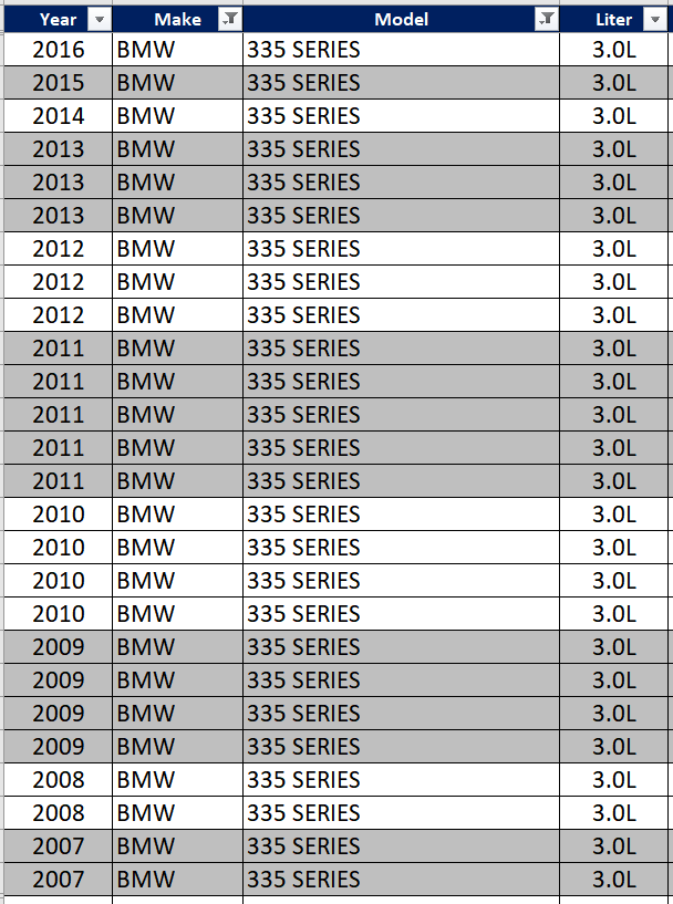
This is what I have in Excel:
excel_have.png


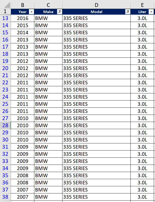
This is what I want:

excel_want.png


I want to highlight the rows at each year change. I am assuming I would need to use Conditional Formatting but do not know what to use for a formula.

I tried google but came up empty on this.

Thanks.
 

Gasman

Enthusiastic Amateur
Local time
Today, 06:02
Joined
Sep 21, 2011
Messages
14,048
Someone just asked the same question for a subform.
arnelgp used the Mod operator in conditional formatting.


EzGoingKev

Registered User.
Local time
Today, 02:02
Joined
Nov 8, 2019
Messages
178
He is doing it in Access on a form. I had to change it up some for Excel.

I used =MOD($B1,2)=0 and selected the Fill option under Format.

Thanks.
 
Last edited:

Isaac

Lifelong Learner
Local time
Yesterday, 23:02
Joined
Mar 14, 2017
Messages
8,738
Use conditional formatting on row 2. Use a formula to determine. (if this is different than that).
then copy it - then paste formats to the rest of the cells. they will paste relative
 

Gasman

Enthusiastic Amateur
Local time
Today, 06:02
Joined
Sep 21, 2011
Messages
14,048
Use conditional formatting on row 2. Use a formula to determine. (if this is different than that).
then copy it - then paste formats to the rest of the cells. they will paste relative
I was thinking just odd and even years?
 

Isaac

Lifelong Learner
Local time
Yesterday, 23:02
Joined
Mar 14, 2017
Messages
8,738
I was thinking just odd and even years?
Yeah, that might give him the overall result he wants, too, not sure

For static sheets I always use that method I posted, as it's so simple. although the majority of my work is automation so I write vba to loop and do it that way

Probably a handful of ways to do it I guess, never heard of MOD with Format Fill, interesting
 

EzGoingKev

Registered User.
Local time
Today, 02:02
Joined
Nov 8, 2019
Messages
178
Yeah, that might give him the overall result he wants, too, not sure

For static sheets I always use that method I posted, as it's so simple. although the majority of my work is automation so I write vba to loop and do it that way

Probably a handful of ways to do it I guess, never heard of MOD with Format Fill, interesting
I ran into an issue.

In my formula of =MOD($B1,2)=0 the 2 is selecting cells containing even numbers. If I change the 2 to a 1 it select cells containing odd numbers.

Audi makes an A3 model that came with a 2.0 liter engine. They dropped the 2.0 liter in 2014 and then picked it back up again. Here is what my data looks like:

audi_2014_issue.png


Because both 2015 and 2013 are odd numbers they do not get highlighted.

Ideally 2015 would stay as is. 2013 would be shaded. 2012 would not be shaded. It would carry all the way down.

Any ideas?
 

Gasman

Enthusiastic Amateur
Local time
Today, 06:02
Joined
Sep 21, 2011
Messages
14,048
So go with Isaac's solution, compare to previous row?
I ran into an issue.

In my formula of =MOD($B1,2)=0 the 2 is selecting cells containing even numbers. If I change the 2 to a 1 it select cells containing odd numbers.

Audi makes an A3 model that came with a 2.0 liter engine. They dropped the 2.0 liter in 2014 and then picked it back up again. Here is what my data looks like:

View attachment 98382

Because both 2015 and 2013 are odd numbers they do not get highlighted.

Ideally 2015 would stay as is. 2013 would be shaded. 2012 would not be shaded. It would carry all the way down.

Any ideas?
 

Isaac

Lifelong Learner
Local time
Yesterday, 23:02
Joined
Mar 14, 2017
Messages
8,738
I thought you wanted it to highlight when it changed. You'd have to sort it first
 

Gasman

Enthusiastic Amateur
Local time
Today, 06:02
Joined
Sep 21, 2011
Messages
14,048
No, the issue is a missing year, which leaves two years together with same colour/non colour?
 

Gasman

Enthusiastic Amateur
Local time
Today, 06:02
Joined
Sep 21, 2011
Messages
14,048
Had a think about this and knocked up the code below.
You will need to test it fully and adjust to suit. I just did a quick test on a few rows I set up. it can be tweaked a lot more.
Code is for the logic only really

Code:
Sub FillAlternateData()
Dim lngStart As Long, lngEnd As Long, lngSave As Long
Dim strValue As String, strLastColumn As String
Dim blnFill As Boolean

strLastColumn = "H"
lngEnd = 1

Range("A1").Select
Do While ActiveCell.Value <> ""
    lngStart = lngEnd
    strValue = ActiveCell.Value
    Do While strValue = ActiveCell.Value
        ActiveCell.Offset(1, 0).Select
    Loop
    lngSave = ActiveCell.Row
    If blnFill Then
        FillRange "A" & lngStart & ":" & strLastColumn & lngSave - 1, "A" & lngSave
    End If
    lngEnd = lngSave
    blnFill = Not blnFill
Loop
End Sub
Sub FillRange(strRange As String, strSave As String)
' Fill range with a colour
' Need strSave as it affects the activecell row

    Range(strRange).Select
    With Selection.Interior
        .Pattern = xlSolid
        .PatternColorIndex = xlAutomatic
        .Color = 65535
        .TintAndShade = 0
        .PatternTintAndShade = 0
    End With
    Range(strSave).Select
End Sub
1645261511323.png
 

Isaac

Lifelong Learner
Local time
Yesterday, 23:02
Joined
Mar 14, 2017
Messages
8,738
No, the issue is a missing year, which leaves two years together with same colour/non colour?

Well if the requirements really had been whenever it changed, then two colors together would be fine. Because it changed twice

It's a matter of stating the requirements in writing correctly from the beginning, rather than just posting a picture sloppy and hoping people read your mind.
 

Gasman

Enthusiastic Amateur
Local time
Today, 06:02
Joined
Sep 21, 2011
Messages
14,048
It's a matter of stating the requirements in writing correctly from the beginning, rather than just posting a picture sloppy and hoping people read your mind.
Now when do we get that? :)
 

Slap

Registered User.
Local time
Today, 06:02
Joined
May 21, 2011
Messages
41
Based on the OP last post this may not be solved, so here is my take:

Code:
Sub groupShader()
    Dim shadeArray, currentShade, thisRow
    Dim criteriaCol As Double, startRow, endRow
    Dim dataArea
    'below if only using alternate colouring
    'shadeArray = Array(xlNone, 3)
    'below for multiple coloured rows
    shadeArray = Array(xlNone, 35, 34, 36, 37)
    currentShade = 0
    'Change below to = X where X is a static column number
    criteriaCol = Application.InputBox("Color on which column number?")
    startRow = 2
    endRow = Cells(Rows.Count, criteriaCol).End(xlUp).Row
    Set dataArea = Cells(startRow, criteriaCol).CurrentRegion
    For thisRow = startRow To endRow
        If thisRow <> startRow Then
            If Cells(thisRow, criteriaCol).Value <> Cells(thisRow - 1, criteriaCol).Value Then
                currentShade = (currentShade + 1) Mod (UBound(shadeArray) + 1)
            End If
        End If
        Intersect(Rows(thisRow), dataArea).Interior.ColorIndex = shadeArray(currentShade)
    Next thisRow
End Sub

Depending on requirement you can alter the number colours and the specific column or allow a choice to be made.

Slap
 

Gasman

Enthusiastic Amateur
Local time
Today, 06:02
Joined
Sep 21, 2011
Messages
14,048
Its has been a few weeks now and no response from OP :(
 

Users who are viewing this thread

Top Bottom