Conditional formatting - using data bars in excel (1 Viewer)

Is there a way to format a data bar (inside a cell) with more than two colors?
I can get the bars to appear green for positive values and red for negative values, but is it possible to show colors for other value ranges?
Eg
Value below 0 = Red
Value between 0 – 20 = Orange
Value between 20 -50 = Green
Value above 50 = Blue

Assuming Excel 2010 and that the Menu is used.
http://www.techonthenet.com/excel/questions/cond_format1_2010.php
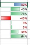
Select the Ragne of cells for the tri-color
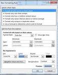
Follow this but instead of the Greater than > choose the rule Between
Then reselect the range of cells again.
Skip to the step of Manage Rules
From here you can Add the two other colors. This allows you to see all of the values so that there is not any cross over.

This is using the wizard, great tool for beginners.

There is a disadvantage to using the wizard:
In my case, Datamining against a database can produce large Excel worksheets of tens of thousands of rows with conditional formatting on 20 columns.
This can add up to 10K rows * 20 columns * 4 rule colors per cell = 800,000 Conditional Format rule caculations. These kind of limits can affect any worksheet change in an unexpected way.

When useing VBA to evaluate the same process one time during the worksheet creation (as the data is pulled in using VBA automation) the worksheet can be set up with zero Conditional Formatting rules.

If only small sets of data are used, no real problem.
If the project takes on many Conditional Formats on larger data sets, consider a different approach.

Not sure what you mean by data bars?, but I've coloured the cells using conditional formatting and individual rules, just as you have listed. So you would just create 4 rules for your criteria.

If this is not what you are asking, then my apologies.

Thank-you for your replies.

FYI. A data bar is a bar chart inside a cell to provide a graphic display of the value of that cell only (vs a chart that displays a series of values).

attached is a screenshot example with the options (see dialog box) that are available.

thanks Rx, for your reply,
it seems to work for formatting cell content (fill/font color)
but I'm not sure it can be applied to data bars?

Ah, OK I see what you are talking about now.

A quick google produced https://www.google.co.uk/webhp?sour...v=2&ie=UTF-8#q=multi coloured data bars excel

and one of the links appears to do what you want?

https://blogs.office.com/2006/02/24/conditional-formatting-trick-1-multi-coloured-data-bars/

This post https://digimac.wordpress.com/2014/06/29/multicoloured-data-bars-in-excel/ appears to refer to the one above, but gives more detail on how to achieve the multi colours.?

HTH

martinr said:

Thank-you for your replies.

FYI. A data bar is a bar chart inside a cell to provide a graphic display of the value of that cell only (vs a chart that displays a series of values).

attached is a screenshot example with the options (see dialog box) that are available.

Click to expand...

DOH! Data Bars. Sorry about that.
Was focused on the English Pubs where Access Programmers hung out (different thread).
I will have to take a look at those last links after my deadline at work is delivered.
Of course, after the deadline, I might go to the Data Bars to celebrate.